
This group project is a collective effort, with contributions from my teammates Minn Thit Aung, Polly Nightingale, Simon Kent, and Xavier Dunn, listed alphabetically.
This post aims to:
- Determine the the basic reproduction number (R0) of an hypothetical outbreak
- Assess the impact of various strategies for vaccination and school closures on accumulative cases and peak cases/timing
- Provide instructions for constructing a SEIR model using Berkeley Madonna
- Offer simple R code for converting a ggplot into a GIF
Setting the Scene
Many countries have recently experienced the first wave of an influenza pandemic caused by the strain HuNz. Now, there are rumours that in a distant country N, the second wave of the pandemic is just starting, and more infections have been reported so far.
The Ministry of Health in country P has become concerned and has called an emergency meeting to discuss the next steps, assuming that the transmissibility of the virus increases by 50% between the first and second waves.
If you were a group of modelling experts in the country P, how do you prepare for this emergency meeting and inform the Ministry of Health the decision-making process?
Model Structure
The type of model used is a deterministic model with an SEIR framework, short for Susceptible-Exposed-Infectious-Removed. This model uses differential equations to estimate the change in populations over time (rate) in the various compartments, assuming static patterns.
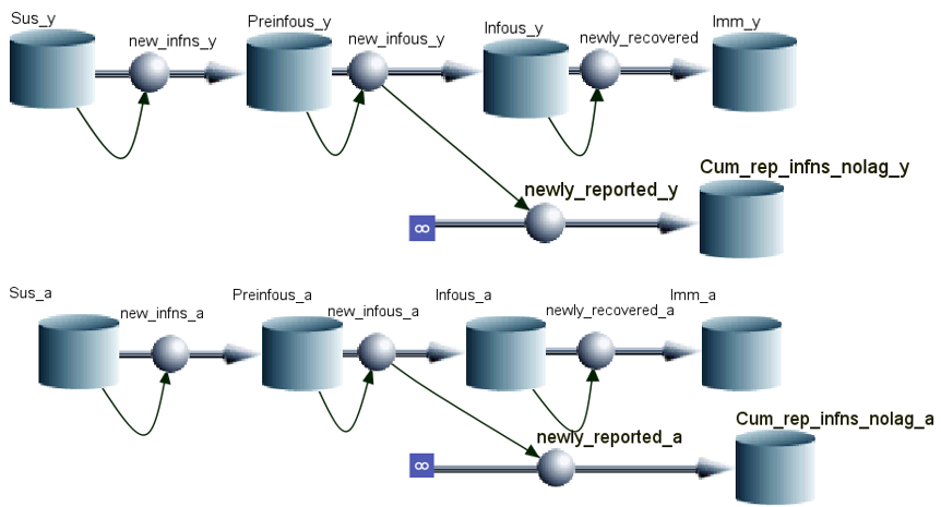
Notably, we incorperate age-dependednt mixing, which means the transmission probability/parameter are different between age groups: children-to-children, adults-to-children, children-to-adults, and adults-to-adults.
Fitting the First Wave
The information already known during the first wave includes: population (182,091 children and 369,909 adults), infectious period (2 days), latent period (2 days), fraction of symptom (60%), fraction of reporting (15%), vaccine efficacy (25%), susceptibility (50% first-wave infected individuals are fully protected against the second strain). Also, through the surveillance system, we’ve known the cummulative weekly number of reported infections for children and adults.
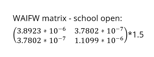
We must ascertain the basic reproductive number (R0) to inform our modelling for the second wave. Using the information mentioned, we apply the Curve Fit function in the Berkeley Madonna to fit our model to the first-wave data. Here comes the the optimal age-dependet transmission parameters: β1, β2, and β3 in the Who-Acquire-Infections-From-Whom (WAIFW) matrix. β is the per capita rate at which two individuals, in this case age-speceficly, come into effective contact per unit time.
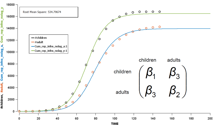
To derive the R0 in the first wave, Next Generation Matrix is used along with a simulation process. Briefly, based on the initial assumed conditions, this method simulate the dynamics of the disease spread over time, i.e. from one generation to the next generation. Once the simulation has reached a steady state (equilibrium), we can estimate R0 using the observed data. Finally we get 1.47 as our R0 in the first wave, which is not far from the historical R0 of influenza in the 20s century.
Modelling for Second Wave
No Intervention
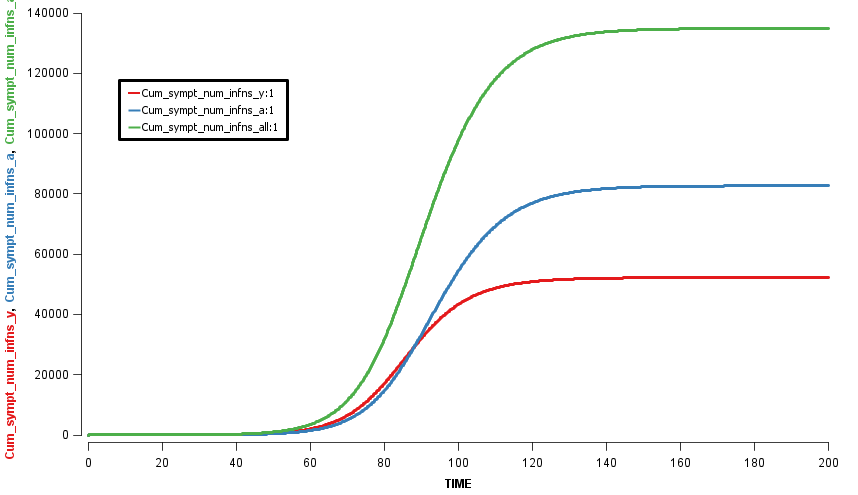
Assuming an initial case of one child infection (seeding) in our country and 100% fraction of reporting, we multiply the first-wave WAIFW matrix by 1.5 because the transmissibility of the second wave is believed to be 50% higher. The Berkeley Madonna SEIR model produces cruves of cumulative number of symptomatic cases of children, adults, and all population.
This is a no-intervention scenario (scenario 1). It is estimated that 28.7% children, 22.3% adults, and 24.4% total population will experience symptoms due to the new influenza strain.
Interventions
Due to a global shortage, we have no stocks of antivirals and hope that closing schools and vaccination will help limit the spread of the infection. However, the vaccines supplied for the second wave are limited and we are expected to receive enough doses for 50% of the population. The available vaccine doses will be given to children, with any remaining doses being given to adults.
The school-closure intervention will shut down the school for four weeks once the true proportion of children who have experienced symptoms during the second wave has reached 0.5%, which is called the school-closure threshold. We suppose that the β1 will be 60% lower during the school-closure period, i.e. the β1 need to be multiplied with 0.4.
In the global environment of the Berkeley Madonna model:

b1_school_open = 5.83845e-6
b1_school_closure = 2.33538e-6
b1 = if ((time> 53) and (time<83)) then b1_school_closure else b1_school_open

where on the 54th day the true proportion of children who have experienced symptoms hit the threshold
Now we can try the modelling for four basic scenrios:
- Scenario 1: No intervention
- Scenario 2: School Closure
- Scenario 3: Vaccination for 100% children and 25.39% adults (=50% total population)
- Scenario 4: Vaccination and School Closure, scenario 2 and 3 combined
Owing to interventions, the proportion symptomatic in the total population are 24.1%, 19.8%, and 19.4% in scenarios 2, 3, and 4, respectively. It can be observed that the impact of school closure is limited, compared to vaccination programme.
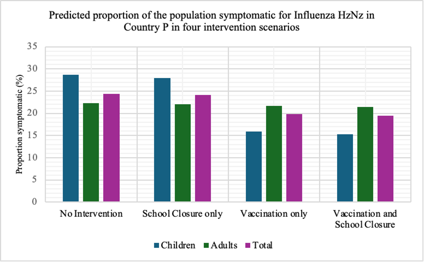
In terms of flatting the curve and delaying the peak, similarly, the vaccination programme performs better than school closure does. The most effective strategy for controlling the outbreak involves a combination of vaccination and school closure measures (scenario 4).
 The R code for this animation is included in the appendix at the bottom.
It is worth examining the Net Reproductive Number (Rn) at various point of time, calculated as the product of the transmission rate (β) with the susceptible population and the duration of infectiousness using the next generation matrix. In the begining of the scenario 1&2, the Rn is 1.59. However, at the first day of the school closure in scenario 2, the Rn decreases to 1.155.
With the collective protection from vaccination and acquired immunity from the first wave, the Rn in the begining of the scenario 3&4 is 1.32. Upon the implementation of school closure in scenario 4, Rn becomes 1.164. The Rn reaches a critical value of one at the peak of each curve.
Sensitivity Analysis
To explore the potential strategies in response to the outbreak, we come up with the following advanced scenarios:
- Scenario 5: Longer School closure (3 months)
- Scenario 6a: Adjsut the threshold of school closure from 0.5% to 0.2%.
- Scenario 6b: Adjsut the threshold of school closure from 0.5% to 1%.
- Scenario 7: Equal vaccine distribution: distribute the same doses vaccines to children and adults.
- Scenario 8: The strain is 200% higher transmissible than the first wave
- Scenario 9: Adjust the fraction of reporting from 100% to 60%
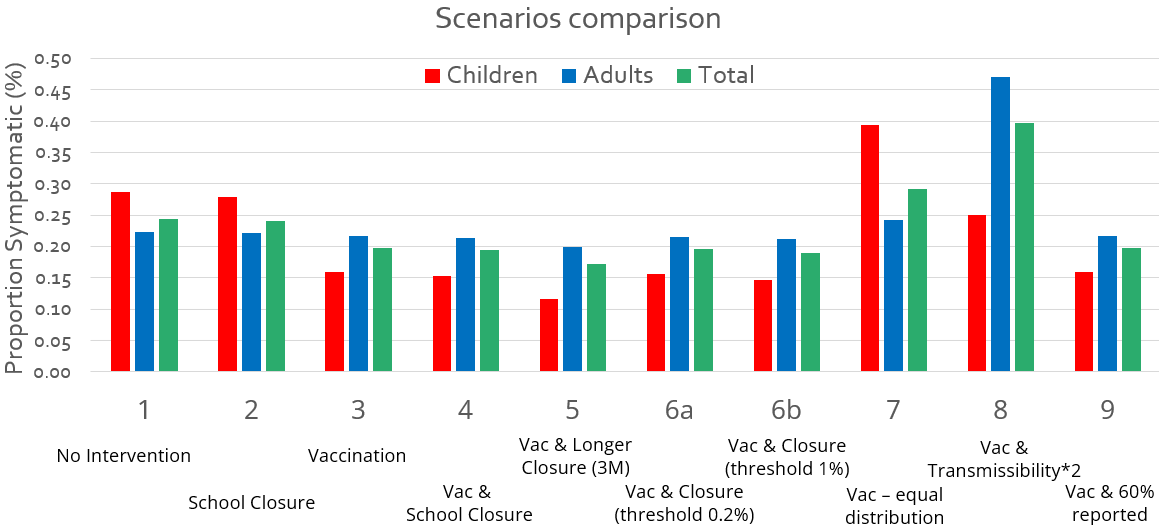
Vaccination Distribution: Equity or Equality?
We regard scenario 3 as a equitable strategy for vaccine distribution, as it prioritize individuals who are more vulnerable to the disease and have a higher transmission rate (where β1 > β2 > β3).
In contrast, scenario 7 is a equal strategy for vaccine distribution. This is a equal allocation due to the same weight (number of vaccine doses) given to both groups of people.
It can be observed that an equitable vaccine distribution program proves more effective in controlling outbreaks compared to equal distribution models, this is due to the equity-driven resource allocation favoring people with higher transmission rates (β1).
Thresholds for School Closure
Apart from proportion symptomatic, peak cases and peak timing are also critical indicators for controlling an outbreak.
| Scenarios | Peak Cases | Peak Day | Prop. Symp. |
|---|---|---|---|
| 8-Vac&200%Trans | 20,917 | 52 | 40% |
| 7-Vac (equal) | 9,597 | 65 | 29% |
| 1-No interv. | 6,077 | 87 | 24% |
| 2-Clos.(0.5%) | 5,298 | 113 | 24% |
| 3-Vac | 3,243 | 140 | 20% |
| 6a-Vac&Clos.(0.2%) | 3,077 | 155 | 20% |
| 4-Vac&Clos.(0.5%) | 2,839 | 156 | 19% |
| 6b-Vac&Clos.(1%) | 2,499 | 157 | 19% |
| 9-Vac&60%Rep. | 1,946 | 140 | 20% |
| 5-Vac&Clos.(3m) | 1,462 | 151 | 17% |
In this table, we sort the scenarios by the peak cases, and we focus on three scenarios with vaccination and different thresholds for school closure (scenario 6a, 4, and 6b). These three scenarios have similar peak timing and proportion symptomatic. However, the higher the threshold we set, the lower the peak cases we have.
In other words, as long as we know the surge capacity of the healthcare system, we can manipulate the threshold to flatten the curve, preventing the health care systems from overwhelming patients.
Conclusion
Key Finding
Choosing from four basic scenarios (1-4), we recommened the vaccination only strategy to our Ministry of Health to mitigate the surges in influenza cases.
In scenario 4, the combined effects of vaccination and school closure result in the largest reduction of symptomatic cases (20.6%) compared to scenario 1 as the reference. However, closing schools may delay the peak of cases, while the significance depends on whether burden to health services, given zero mortality in this context.
Cost to society of school closure may result in disrupting children’s education/causing parents to miss work. This highlights the importance of considering the Incremental Cost Effectiveness Ratio (ICER) in the modelling.
Limitations
This hypothetical study has some limitations due to the assumptions. First, no births or deaths are included in model. Second, we assume the latent and infectious periods in the second wave are the same as virus in first wave. Third, proportions of cases showing symptoms is assumed the same in adults and children, and the fraction of reporting is not possible to reach 100% in the realworld settings.
Recommendations
First of all, it’s important to collect more data to conduct a more comprehensive economic evaluation of control measures, which is the highlighted in a panel discussion at LSHTM - The use of modelling to inform decision-making in an emergency: lessons from COVID-19. Assessing changes in behavior throughout an outbreak in real-time can be challenging as they are difficult to predict in advance. Besides, assessing the effects on healthcare service is critial. It may also be useful to conduct a cohort/surveillance that we study for seroprevalence through outbreaks. The Ministry of Health may try to combine other non-pharmaceutical interventions, e.g. social distancing, wearing mask, personal hygiene.
This group project was originally intended for a group presentation of the the Modelling and the Dynamics of Infectious Diseases module at LSHTM, with contributions from Minn Thit Aung, Polly Nightingale, Simon Kent, and Xavier Dunn, listed alphabetically.
Appendix
# The gganimate package demonstrates how to make the ggplot in the scenario 1-4 into a GIF
#The data structure should be: a day of newly reported cases in each row, and each column is a scenario

library(gganimate)

plot_object <- ggplot() +
geom_line(data=df1,aes(x=Time,y=Scenario1),color="#088199",size=0.7)+
geom_line(data=df1,aes(x=Time,y=Scenario2),color="purple",size=0.7)+
geom_line(data=df1,aes(x=Time,y=Scenario3),color="#Ca0020",size=0.7)+
geom_line(data=df1,aes(x=Time,y=Scenario4),color="#b8e186",size=0.7)+
geom_text(data=df1,aes(x=Time, y=Scenario1 + 1.5,label=paste('S1')), color = "#088199")+
geom_text(data=df1,aes(x=Time, y=Scenario2 + 1.5,label=paste('S2')), color = "purple") +
geom_text(data=df1,aes(x=Time, y=Scenario3 + 1.5,label=paste('S3')), color = "#Ca0020")+
geom_text(data=df1,aes(x=Time, y=Scenario4 + 1.5,label=paste('S4')), color = "#b8e186")+
theme(panel.grid.major = element_blank(),
      axis.line = element_line(colour = "black"),
      panel.background = element_rect(fill = "transparent"),
      plot.title=element_text(hjust=0.5)) +
scale_x_continuous(breaks=seq(0,350,25))+
labs(y="Daily New Reported Cases",x = 'Time (Day)',title = "Outbreak Dynamics of Influenza Strain HuNz")

print(plot_object)

plot_object_transition <- plot_object + transition_reveal(Time) # make static into dynamic

animate(plot_object_transition, #save the GIF
        fps = 50, #frame rate
        duration = 1.5, #speed
        width = 1800, height = 865, #dimension
        renderer = gifski_renderer(loop = FALSE,"My_animation.gif"),
        res= 100)# accuracy every fold